Example of Thermo-elastic and electrical coupling (simple nonlinear coupled problem, model object, generic assembly, solve and visualization)
This example aims to present a simple example of a multiphysics problem with a nonlinear coupling of a displacement field, a temperature field and an electric potential field. It also aims to compare the use of the GetFEM C++ API and the GetFEM scripting interfaces. The corresponding demo files are available in the test directories of GetFEM (tests/, interface/tests/python, interface/scr/scilab/demos and interface/tests/matlab).
The problem setting
Let \(\Omega \subset \rm I\hspace{-0.15em}R^2\) be the reference configuration of a 2D plate (see the geometry here) of thickness \(t\) submitted to external forces, electric potential and heating. We will denote by \(T : \Omega \rightarrow \rm I\hspace{-0.15em}R\) the temperature field (in °C), \(V : \Omega \rightarrow \rm I\hspace{-0.15em}R\) the electric potential field and \(u : \Omega \rightarrow \rm I\hspace{-0.15em}R^2\) the in-plane displacement field.
Thermal problem
The left and right sides of the plate as well as the hole surfaces, alltogether denoted with \(\Gamma_i\), are supposed to be in thermal insulation. The bottom and top sides, denoted with \(\Gamma_c\), as well as the front and back faces of the plate are supposed to be in thermal exchange with surrounding air at temperature \(T_{air} = 20\) °C) with a heat transfer coefficient \(D\).
The heat transfer equation for the temperature field \(T\) including all relevant boundary conditions can be written as follows:
where \(\kappa\) is the thermal conductivity and \(n\) the outward unit normal vector to \(\Omega\) on \(\partial \Omega\).
The term \(1/\rho|\nabla V|^2\) is a coupling term corresponding to Joule heating due to electric current, where \(\rho\) is the electric resistivity, hence \(1/\rho\) is the electric conductivity.
Electric potential problem
We consider a potential difference of \(0.1V\) between the left and right lateral faces of the plate. All other faces are considered electrically insulated. The governing equation for the electric potential is
where \(\rho\) is still the electric resistivity. Moreover, we consider that \(\rho\) depends on the temperature as follows:
where \(T_0\) is a reference temperature, \(\rho_0\) the resistivity at \(T_0\) and \(\alpha\) is the resistivity-temperature coefficient.
Deformation problem
We consider the planar deformation of the plate under a force applied on the right lateral face and influenced by the heating of the plate, assuming plane stress conditions. For linearized elasticity the displacement field \(u\) has to satisfy the following equations:
where \(F\) is the force density applied on the right lateral boundary and \(\sigma(u)\) is the Cauchy stress tensor defined by
with \(\varepsilon(u) = (\nabla u + (\nabla u)^T)/2\) being the linearized strain tensor, \(I\) the identity second order tensor, \(E\) and \(\nu\) the Young modulus and Poisson ratio of the material, and \(\alpha_{th}\) the thermal expansion coefficient.
The weak formulation
An important step is to obtain the weak formulation of the coupled system of equations. This is a crucial step since representing PDEs using standard finite element theory relies on their weak formulation (Galerkin approximation).
Weak formulation of each partial differential equation is obtained by multiplying the equation with a test function corresponding to the main unknown. The test function needs to satisfy homogeneous Dirichlet conditions everywhere where the main unknown is prescribed by a Dirichlet condition. Then integrating over the domain \(\Omega\) and performing some integrations by parts (using Green’s formula) leads to the weak formulation of the system of partial differential in the form:
where \(\delta T, \delta V, \delta u\) are the test functions corresponding to \(T, V, u\), respectively, \(\Gamma_N\) denotes the right boundary where the density of force \(F\) is applied and \(\sigma:\varepsilon\) is the Frobenius scalar product between second order tensors.
Implementation in C++ and in script languages
Let us now make a detailed presentation of the use of GetFEM to approximate the problem. We build simultaneously a C++, Python, Scilab and Matlab program. In the scripts for Matlab/Octave we choose not to make use of the object oriented syntax (see GetFEM OO-commands on how to use the OO syntax and its computational overhead).
Initialization
First, in C++, ones has to include a certain number of headers for the model object, the generic assembly, the experimental mesher, and the export functionality. For Python, GetFEM can just be imported globally, and typically numpy needs to be imported as well. For Scilab, the library has first to be loaded in the Scilab console (this is not described here) and for Matlab/Octave, it is only recommended to call gf_workspace(‘clear all’) to ensure there are no leftover GetFEM variables in memory.
C++ |
#include "getfem/getfem_model_solvers.h"
#include "getfem/getfem_export.h"
#include "getfem/getfem_mesher.h"
#include "getfem/getfem_generic_assembly.h"

using std::cout; using std::endl;
using bgeot::dim_type;
using bgeot::size_type;
using bgeot::base_node;
using bgeot::base_small_vector;

int main() {
|
Python |
import getfem as gf
import numpy as np
|
Matlab, Octave, Scilab |
gf_workspace('clear all');
|
Parameters of the model
Let us now define the different physical and numerical parameters of the problem. For script languages (Python, Matlab/Octave, and Scilab) exactly the same syntax can be used.
C++ |
double t = 1.,            // Thickness of the plate (cm)
       E = 21E6,          // Young Modulus (N/cm^2)
       nu = 0.3,          // Poisson ratio
       F = 100E2,         // Force density at the right boundary (N/cm^2)
       kappa = 4.,        // Thermal conductivity (W/(cm K))
       D = 10.,           // Heat transfer coefficient (W/(K cm^2))
       air_temp = 20,     // Temperature of the air in deg C.
       alpha_th = 16.6E-6,// Thermal expansion coefficient (1/K)
       T0 = 20.,          // Reference temperature in deg C
       rho_0 = 1.754E-8,  // Resistivity at T0
       alpha = 0.0039;    // Resistivity-temperature coefficient

double h = 2.                 // Approximate mesh size
dim_type elements_degree = 2; // Degree of the finite element methods
|
Scripts |
t = 1.; E = 21E6; nu = 0.3; F = 100E2;
kappa = 4.; D = 10.; air_temp = 20.; alpha_th = 16.6E-6;
T0 = 20.; rho_0 = 1.754E-8; alpha = 0.0039;

h = 2.; elements_degree = 2;
|
Mesh generation
GetFEM has some limited mesh generation capabilities which are described here. However, GetFEM is not meant to be used as a general purpose mesher, there is no guaranty of the quality and conformity of the obtained mesh. You should better always verify the quality of the generated mesh if you use GetFEM’s built-in meshing tools. You can also use external meshers like GMSH, ANSYS, or GiD, and import the generated meshes (see Save and load meshes).
The geometry of the domain in the present example is a rectangle with three circular holes (see The obtained mesh.).
The mesh for this geometry is produced by combining geometrical primitives with boolean operations (see src/getfem/getfem_mesher.h file).
In the following, h stands for the mesh size and 2 is the degree of the mesh (this means that the transformation is of degree two, we used curved edges). In order to get isoparametric elements, the parameter elements_degree, used later in the definition of finite element spaces, needs also to be set equal to 2. Otherwise subparametric or superparametric elements will be produced.
C++ |
getfem::mesh mesh;
getfem::pmesher_signed_distance
  mo1 = getfem::new_mesher_rectangle(base_node(0., 0.), base_node(100., 25.)),
  mo2 = getfem::new_mesher_ball(base_node(25., 12.5), 8.),
  mo3 = getfem::new_mesher_ball(base_node(50., 12.5), 8.),
  mo4 = getfem::new_mesher_ball(base_node(75., 12.5), 8.),
  mo5 = getfem::new_mesher_union(mo2, mo3, mo4),
  mo = getfem::new_mesher_setminus(mo1, mo5);

std::vector<getfem::base_node> fixed;
getfem::build_mesh(mesh, mo, h, fixed, 2, -2);
|
Python |
mo1 = gf.MesherObject('rectangle', [0., 0.], [100., 25.])
mo2 = gf.MesherObject('ball', [25., 12.5], 8.)
mo3 = gf.MesherObject('ball', [50., 12.5], 8.)
mo4 = gf.MesherObject('ball', [75., 12.5], 8.)
mo5 = gf.MesherObject('union', mo2, mo3, mo4)
mo  = gf.MesherObject('set_minus', mo1, mo5)

mesh = gf.Mesh('generate', mo, h, 2)
|
Matlab, Octave, Scilab |
mo1 = gf_mesher_object('rectangle', [0 0], [100 25]);
mo2 = gf_mesher_object('ball', [25 12.5], 8);
mo3 = gf_mesher_object('ball', [50 12.5], 8);
mo4 = gf_mesher_object('ball', [75 12.5], 8);
mo5 = gf_mesher_object('union', mo2, mo3, mo4);
mo  = gf_mesher_object('set_minus', mo1, mo5);

mesh = gf_mesh('generate', mo, h, 2);
|
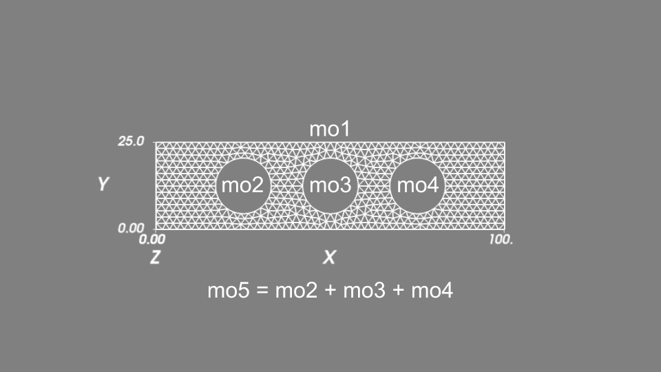
The obtained mesh.
Boundary selection
Since we have different boundary conditions on the different parts of the boundary, we have to number different parts of the boundary accordingly. Sets of elements or element faces on the mesh are defined in so called mesh regions (see Mesh regions) with a unique integer identifier. Regions with identifiers 1, 2, 3, and 4 are defined for the right, left, top and bottom sides, respectively. These boundary numbers will be used in the definitions of different terms in the model equations.
C++ |
getfem::mesh_region border_faces;
getfem::outer_faces_of_mesh(mesh, border_faces);
getfem::mesh_region
   fb1 = getfem::select_faces_in_box(mesh, border_faces,
                                     base_node(1., 1.), base_node(99., 24.)),
   fb2 = getfem::select_faces_of_normal(mesh, border_faces,
                                        base_small_vector( 1., 0.), 0.01),
   fb3 = getfem::select_faces_of_normal(mesh, border_faces,
                                        base_small_vector(-1., 0.), 0.01),
   fb4 = getfem::select_faces_of_normal(mesh, border_faces,
                                        base_small_vector(0.,  1.), 0.01),
   fb5 = getfem::select_faces_of_normal(mesh, border_faces,
                                        base_small_vector(0., -1.), 0.01);

size_type RIGHT_BOUND=1, LEFT_BOUND=2, TOP_BOUND=3, BOTTOM_BOUND=4;
mesh.region( RIGHT_BOUND) = getfem::mesh_region::subtract(fb2, fb1);
mesh.region(  LEFT_BOUND) = getfem::mesh_region::subtract(fb3, fb1);
mesh.region(   TOP_BOUND) = getfem::mesh_region::subtract(fb4, fb1);
mesh.region(BOTTOM_BOUND) = getfem::mesh_region::subtract(fb5, fb1);
|
Python |
fb1 = mesh.outer_faces_in_box([1., 1.], [99., 24.])
fb2 = mesh.outer_faces_with_direction([ 1., 0.], 0.01)
fb3 = mesh.outer_faces_with_direction([-1., 0.], 0.01)
fb4 = mesh.outer_faces_with_direction([0.,  1.], 0.01)
fb5 = mesh.outer_faces_with_direction([0., -1.], 0.01)

RIGHT_BOUND=1; LEFT_BOUND=2; TOP_BOUND=3; BOTTOM_BOUND=4; HOLE_BOUND=5;

mesh.set_region( RIGHT_BOUND, fb2)
mesh.set_region(  LEFT_BOUND, fb3)
mesh.set_region(   TOP_BOUND, fb4)
mesh.set_region(BOTTOM_BOUND, fb5)
mesh.set_region(  HOLE_BOUND, fb1)
mesh.region_subtract( RIGHT_BOUND, HOLE_BOUND)
mesh.region_subtract(  LEFT_BOUND, HOLE_BOUND)
mesh.region_subtract(   TOP_BOUND, HOLE_BOUND)
mesh.region_subtract(BOTTOM_BOUND, HOLE_BOUND)
|
Matlab, Octave, Scilab |
fb1 = gf_mesh_get(mesh, 'outer_faces_in_box', [1 1], [99 24]);
fb2 = gf_mesh_get(mesh, 'outer_faces_with_direction', [ 1 0], 0.01);
fb3 = gf_mesh_get(mesh, 'outer_faces_with_direction', [-1 0], 0.01);
fb4 = gf_mesh_get(mesh, 'outer_faces_with_direction', [0  1], 0.01);
fb5 = gf_mesh_get(mesh, 'outer_faces_with_direction', [0 -1], 0.01);

RIGHT_BOUND=1; LEFT_BOUND=2; TOP_BOUND=3; BOTTOM_BOUND=4; HOLE_BOUND=5;
gf_mesh_set(mesh, 'region',  RIGHT_BOUND, fb2);
gf_mesh_set(mesh, 'region',   LEFT_BOUND, fb3);
gf_mesh_set(mesh, 'region',    TOP_BOUND, fb4);
gf_mesh_set(mesh, 'region', BOTTOM_BOUND, fb5);
gf_mesh_set(mesh, 'region',   HOLE_BOUND, fb1);
gf_mesh_set(mesh, 'region_subtract',  RIGHT_BOUND, HOLE_BOUND);
gf_mesh_set(mesh, 'region_subtract',   LEFT_BOUND, HOLE_BOUND);
gf_mesh_set(mesh, 'region_subtract',    TOP_BOUND, HOLE_BOUND);
gf_mesh_set(mesh, 'region_subtract', BOTTOM_BOUND, HOLE_BOUND);
|
Mesh draw
In order to preview the mesh and verify its quality, the following instructions can be used:
C++ |
getfem::vtu_export exp("mesh.vtu", false);
exp.exporting(mesh);
exp.write_mesh();
// You can view the mesh for instance with
// mayavi2 -d mesh.vtu -f ExtractEdges -m Surface
|
Python |
mesh.export_to_vtu('mesh.vtu');
# You can view the mesh for instance with
# mayavi2 -d mesh.vtu -f ExtractEdges -m Surface
|
Matlab, Octave, Scilab |
scf(1);
gf_plot_mesh(mesh, 'refine', 8, 'curved', 'on', 'regions', ...
             [RIGHT_BOUND LEFT_BOUND TOP_BOUND BOTTOM_BOUND]);
title('Mesh');
|
For Matlab/Octave call pause(1); and for Scilab call sleep(1000); just after.
In C++ and with the Python interface, an external graphical post-processor has to be used (for instance, gmsh, Mayavi2, PyVista or Paraview). With Scilab and Matlab/Octave interfaces, the internal plot facilities can be used (see the result The obtained mesh.).
Definition of finite element methods and integration method
We will define three finite element methods. The first one, mfu, is to approximate the displacement field which is a vector field. Its definition in C++ is
getfem::mesh_fem mfu(mesh, 2);
mfu.set_classical_finite_element(elements_degree);
where the argument 2 stands for the dimension of the vector field. The second line sets the finite element used, where classical_finite_element means a continuous Lagrange element. Remember that elements_degree has been set to 2 which means that we will use quadratic (isoparametric) elements.
There is a wide choice of pre-existing finite element methods in GetFEM, see Appendix A. Finite element method list. However, Lagrange finite element methods are the most common in practice.
The second finite element method is a scalar one, mft, which will approximate both the temperature and the electric potential fields. Several finite element variables can share the same finite element method if necessary.
The third finite element method, mfvm, is a discontinuous Lagrange one for a scalar field, which will allow us to post-process quantities which are discotinuous at element boundaries, such as the gradient of some approximated field variables, in particular the Von Mises stress field.
The last thing to define is an integration method mim. There is no default integration method in GetFEM, so it is mandatory to define an integration method. Of course, the order of the integration method has to be chosen sufficient large to provide full integration of the relevant finite element terms. In the present example, a polynomial order equal to the double of elements_degree is sufficient.
C++ |
getfem::mesh_fem mfu(mesh, 2);
mfu.set_classical_finite_element(elements_degree);
getfem::mesh_fem mft(mesh, 1);
mft.set_classical_finite_element(elements_degree);
getfem::mesh_fem mfvm(mesh, 1);
mfvm.set_classical_discontinuous_finite_element(elements_degree);

getfem::mesh_im  mim(mesh);
mim.set_integration_method(2*elements_degree);
|
Python |
mfu = gf.MeshFem(mesh, 2)
mfu.set_classical_fem(elements_degree)
mft = gf.MeshFem(mesh, 1)
mft.set_classical_fem(elements_degree)
mfvm = gf.MeshFem(mesh, 1)
mfvm.set_classical_discontinuous_fem(elements_degree)
mim = gf.MeshIm(mesh, elements_degree*2)
|
Matlab, Octave, Scilab |
mfu = gf_mesh_fem(mesh, 2);
gf_mesh_fem_set(mfu, 'classical_fem', elements_degree);
mft = gf_mesh_fem(mesh, 1);
gf_mesh_fem_set(mft, 'classical_fem', elements_degree);
mfvm = gf_mesh_fem(mesh, 1);
gf_mesh_fem_set(mfvm, 'classical_discontinuous_fem', elements_degree-1);
mim = gf_mesh_im(mesh, elements_degree*2);
|
Model definition
It is not strictly mandatory to use the model object in GetFEM, but it is indeed a very powerful object. It is used to gather all defined variables (unknowns) and data, whether these are defined in a finite element space, on integration points, or globally. It also gathers all PDE terms that involve the various variables and data, numbers the degrees of freedom from all unknowns, and combines all assembled terms into a global tangent system consistently.
For each model object, the user can add predefined PDE terms, so-called model bricks, or preferably add linear/nonlinear terms using symbolic expressions written in the generic weak form language (GWFL) (see Compute arbitrary terms - high-level generic assembly procedures - Generic Weak-Form Language (GWFL)). The added terms can involve a single variable or several variables with arbitrary couplings. The model object automates the assembly of the (tangent) linear system (see The model object for more details).
The alternative to using the model object is to use lower-level assembly procedures directly and incorporate their results into the overall (tangent) linear system manually. However, it is generally highly recommended to use the framework of the model object, as it allows for rapid implementation of a model. All common boundary conditions, PDE terms, multiplier- enforced constraints, etc., can be easily provided in a very compact form as GWFL expressions. Many common terms are predefined in so-called bricks; however, nowadays these are somewhat obsolete, as the use of GWFL is almost as compact and at the same time more transparent. There are a few specific model bricks that act directly on the discretized system, such as the explicit matrix brick and the explicit rhs brick, which provide operations that cannot be expressed in GWFL.
When defining a model object, there are two options to choose from: real-number and complex-number model versions. Complex-number models are reserved for special applications (e.g., some electromagnetism problems) where it is advantageous to solve a complex-number linear system. They support most, but not all, features available in the real-number model version.
Let us declare a real-number model with the three variables corresponding to the three unknown fields:
C++ |
getfem::model md;
md.add_fem_variable("u", mfu);
md.add_fem_variable("T", mft);
md.add_fem_variable("V", mft);
|
Python |
md=gf.Model('real');
md.add_fem_variable('u', mfu)
md.add_fem_variable('T', mft)
md.add_fem_variable('V', mft)
|
Matlab, Octave, Scilab |
md=gf_model('real');
gf_model_set(md, 'add_fem_variable', 'u', mfu);
gf_model_set(md, 'add_fem_variable', 'T', mft);
gf_model_set(md, 'add_fem_variable', 'V', mft);
|
Plane stress elastic deformation problem
Let us now begin by the elastic deformation problem. We will use the add_linear_term function of the model object to add a linear term to the model by means of a GWFL symbolic expression. Specifically for the plane stress problem we will add the term
to the tangent linear system, with
In order to add this term, global scalar data corresponding to the elastic constants \(E\) and \(\nu\), as well as the constants \(t\), \(T_0\), and \(\alpha_{th}\), have to be added to the model first. If any of these data were not constant, it is also possible to define them as a finite element field or at integration points directly (not shown here). Note that this term, already incorporates the thermomechanical coupling between the displacement and temperature fields. For the isothermal case, one could alternatively also use a predefined brick, a black-box term, added to the model with the add_isotropic_linearized_elasticity_brick function. Terms provided by GWFL expressions are unambigouous, and they are compiled into a list of optimized assembly instructions which are executed on each Gauss point.
The second term to add to the elasticity problem is the external load on the right boundary, corresponding to the term
This term is added to the model using the add_linear_term function with the GWFL expression “-t*F*Test_u(1)”, and the region number RIGHT_BOUND=1. The predefined brick term alternative to this expression would be by using the function add_source_term_brick (not used here).
A predefined brick will be used for the Dirichlet condition on the left boundary. There are several options to prescribe a Dirichlet condition (see Dirichlet condition brick), but here the function add_Dirichlet_condition_with_multipliers will be used. It would be rather easy to achieve the same effect just with an appropriate GWFL expression and the generic add_linear_term function, but the more specific function spares the user from defining the Lagrange multiplier variable, as this is taken care of internally inside the add_Dirichlet_condition_with_multipliers function.
The following snippets show the definition of the entire elastic deformation equation with thermal expansion.
C++ |
md.add_initialized_scalar_data("t", t);
md.add_initialized_scalar_data("E", E);
md.add_initialized_scalar_data("nu", nu);
md.add_initialized_scalar_data("alpha_th", alpha_th);
md.add_initialized_scalar_data("T0", T0);
md.add_macro("sigma", "E/(1+nu)*( nu/(1-nu)*(Div(u)-2*alpha_th*T)*Id(2)"
                      "+(Sym(Grad(u))-alpha_th*T*Id(2)) )");
getfem::add_linear_term(md, mim, "t*sigma:Grad(Test_u)");
getfem::add_Dirichlet_condition_with_multipliers
  (md, mim, "u", elements_degree-1, LEFT_BOUND);
md.add_initialized_scalar_data("F", F);
getfem::add_linear_term(md, mim, "-t*F*Test_u(1)", RIGHT_BOUND);
|
Python |
md.add_initialized_data('t', t)
md.add_initialized_data('E', E)
md.add_initialized_data('nu', nu)
md.add_initialized_data('alpha_th', alpha_th)
md.add_initialized_data('T0', T0)
md.add_macro('sigma',
             'E/(1+nu)*( nu/(1-nu)*(Div(u)-2*alpha_th*T)*Id(2)'
                       '+(Sym(Grad(u))-alpha_th*T*Id(2)) )')
md.add_linear_term(mim, 't*sigma:Grad(Test_u)')
md.add_Dirichlet_condition_with_multipliers(mim, 'u', elements_degree-1, LEFT_BOUND)
md.add_initialized_data('F', F)
md.add_linear_term(mim, '-t*F*Test_u(1)', RIGHT_BOUND)
|
Matlab, Octave, Scilab |
gf_model_set(md, 'add_initialized_data', 't', t);
gf_model_set(md, 'add_initialized_data', 'E', E);
gf_model_set(md, 'add_initialized_data', 'nu', nu);
gf_model_set(md, 'add_initialized_data', 'alpha_th', alpha_th);
gf_model_set(md, 'add_initialized_data', 'T0', T0);
gf_model_set(md, 'add_macro', 'sigma',...
                              ['E/(1+nu)*( nu/(1-nu)*(Div(u)-2*alpha_th*T)*Id(2)'...
                               '+(Sym(Grad(u))-alpha_th*T*Id(2)) )']);
gf_model_set(md, 'add_linear_term', mim, 't*sigma:Grad(Test_u)');
gf_model_set(md, 'add_Dirichlet_condition_with_multipliers', mim, 'u', elements_degree-1, LEFT_BOUND);
gf_model_set(md, 'add_initialized_data', 'F', F);
gf_model_set(md, 'add_linear_term', mim, '-t*F*Test_u(1)', RIGHT_BOUND);
|
Electric potential problem
Similarly, the following snippets define the electric potential equations. Note the definition of the electric resistivity function \(\rho(T)\) as a macro, and again the heavy use of GWFL expression inside the functions add_linear_term and add_nonlinear_term.
C++ |
md.add_initialized_scalar_data("rho_0", rho_0);
md.add_initialized_scalar_data("alpha", alpha);
md.add_macro("rho", "rho_0*(1+alpha*(T-T0))");
getfem::add_nonlinear_term(md, mim, "t/rho * Grad(V).Grad(Test_V)");
getfem::add_Dirichlet_condition_with_multipliers
  (md, mim, "V", elements_degree-1, RIGHT_BOUND);
md.add_initialized_scalar_data("DdataV", 0.1);
getfem::add_Dirichlet_condition_with_multipliers
  (md, mim, "V", elements_degree-1, LEFT_BOUND, "DdataV");
|
Python |
md.add_initialized_data('rho_0', rho_0)
md.add_initialized_data('alpha', alpha)
md.add_macro('rho', 'rho_0*(1+alpha*(T-T0))')
md.add_nonlinear_term(mim, 't/rho * Grad(V).Grad(Test_V)')
md.add_Dirichlet_condition_with_multipliers(mim, 'V', elements_degree-1, RIGHT_BOUND)
md.add_initialized_data('DdataV', 0.1)
md.add_Dirichlet_condition_with_multipliers(mim, 'V', elements_degree-1, LEFT_BOUND, 'DdataV')
|
Matlab, Octave, Scilab |
gf_model_set(md, 'add_initialized_data', 'rho_0', rho_0);
gf_model_set(md, 'add_initialized_data', 'alpha', alpha);
gf_model_set(md, 'add_macro', 'rho', 'rho_0*(1+alpha*(T-T0))');
gf_model_set(md, 'add_nonlinear_term', mim, 't/rho * Grad(V).Grad(Test_V)');
gf_model_set(md, 'add_Dirichlet_condition_with_multipliers', mim, 'V', elements_degree-1, RIGHT_BOUND);
gf_model_set(md, 'add_initialized_data', 'DdataV', 0.1);
gf_model_set(md, 'add_Dirichlet_condition_with_multipliers', mim, 'V', elements_degree-1, LEFT_BOUND, 'DdataV');
|
Thermal problem
Finally, the definition of the thermal problem is done in the following snippets:
C++ |
md.add_initialized_scalar_data("kappaT", kappa);
md.add_initialized_scalar_data("D", D);
md.add_initialized_scalar_data("T_air", air_temp);
getfem::add_linear_term(md, mim,
                        "t*kappaT*Grad(T).Grad(Test_T) + 2*D*(T-T_air)*Test_T");
getfem::add_linear_term(md, mim, "t*D*(T-T_air).Test_T", TOP_BOUND);
getfem::add_linear_term(md, mim, "t*D*(T-T_air).Test_T", BOTTOM_BOUND);
getfem::add_nonlinear_term(md, mim, "-t/rho * Norm_sqr(Grad(V))*Test_T");
|
Python |
md.add_initialized_data('kappaT', kappa)
md.add_initialized_data('D', D)
md.add_initialized_data('T_air', air_temp)
md.add_linear_term(mim, 't*kappaT*Grad(T).Grad(Test_T) + 2*D*(T-T_air)*Test_T')
md.add_linear_term(mim, 't*D*(T-T_air).Test_T', TOP_BOUND)
md.add_linear_term(mim, 't*D*(T-T_air).Test_T', BOTTOM_BOUND)
md.add_nonlinear_term(mim, '-t/rho * Norm_sqr(Grad(V))*Test_T')
|
Matlab, Octave, Scilab |
gf_model_set(md, 'add_initialized_data', 'kappaT', kappa);
gf_model_set(md, 'add_initialized_data', 'D', D);
gf_model_set(md, 'add_initialized_data', 'T_air', air_temp);
gf_model_set(md, 'add_linear_term', mim, 't*kappaT*Grad(T).Grad(Test_T) + 2*D*(T-T_air)*Test_T');
gf_model_set(md, 'add_linear_term', mim, 't*D*(T-T_air).Test_T', TOP_BOUND);
gf_model_set(md, 'add_linear_term', mim, 't*D*(T-T_air).Test_T', BOTTOM_BOUND);
gf_model_set(md, 'add_nonlinear_term', mim, '-t/rho * Norm_sqr(Grad(V))*Test_T');
|
Model solve
Once the model is correctly defined, we can simply solve it by:
C++ |
gmm::iteration iter(1E-9, 1, 100);
getfem::standard_solve(md, iter);
|
Python |
md.solve('max_res', 1E-9, 'max_iter', 100, 'noisy')
|
Matlab, Octave, Scilab |
gf_model_get(md, 'solve', 'max_res', 1E-9, 'max_iter', 100, 'noisy');
|
Since the problem has some nonlinear terms, a Newton method is used to iteratively solve the problem. It takes just a few iterations (about 4 in this case) to converge at the prescribed residual threshold.
Model solve with two steps
Another option to solve the problem is to solve first the thermal and electric potential problems. Indeed, in our model, the thermal and electric potential equations do not depend on the deformation. Once the thermal and electric potential problems are solved, then we can solve the deformation problem. This can be done as follows:
C++ |
gmm::iteration iter(1E-9, 1, 100);
md.disable_variable("u");
getfem::standard_solve(md, iter);
md.enable_variable("u");
md.disable_variable("T");
md.disable_variable("V");
iter.init();
getfem::standard_solve(md, iter);
|
Python |
md.disable_variable('u')
md.solve('max_res', 1E-9, 'max_iter', 100, 'noisy')
md.enable_variable('u')
md.disable_variable('T')
md.disable_variable('V')
md.solve('max_res', 1E-9, 'max_iter', 100, 'noisy')
|
Matlab, Octave, Scilab |
gf_model_set(md, 'disable_variable', 'u');
gf_model_get(md, 'solve', 'max_res', 1E-9, 'max_iter', 100, 'noisy');
gf_model_set(md, 'enable_variable', 'u');
gf_model_set(md, 'disable_variable', 'T');
gf_model_set(md, 'disable_variable', 'V');
gf_model_get(md, 'solve', 'max_res', 1E-9, 'max_iter', 100, 'noisy');
|
Export/visualization of the solution
The finite element problem is now solved. We can plot the solution as follows. Note that for the C++ and Python programs, it is necessary to use an external graphical post-processor. Note also that arbitrary quantities can be post-processed using the generic interpolation (see ga_interpolation_Lagrange_fem below). It is also possible to make complex exports and slices (see Export and view a solution).
C++ |
getfem::model_real_plain_vector VM(mfvm.nb_dof()), CO(mfvm.nb_dof() * 2);
getfem::ga_local_projection // needs a discontinuous mesh_fem
  (md, mim, "sqrt(Norm_sqr(sigma)+sqr(sigma(1,2))-sigma(1,1)*sigma(2,2))",
   mfvm, VM);
getfem::ga_interpolation_Lagrange_fem(md, "-t/rho * Grad(V)", mfvm, CO);

getfem::vtu_export exp("displacement_with_von_mises.vtu", false);
exp.exporting(mfu);
exp.write_point_data(mfu, md.real_variable("u"), "elastostatic displacement");
exp.write_point_data(mfvm, VM, "Von Mises stress");
cout << "\nYou can view solutions with for instance:\n\nmayavi2 "
  "-d displacement_with_von_mises.vtu -f WarpVector -m Surface\n" << endl;

getfem::vtu_export exp2("temperature.vtu", false);
exp2.exporting(mft);
exp2.write_point_data(mft, md.real_variable("T"), "Temperature");
cout << "mayavi2 -d temperature.vtu -f WarpScalar -m Surface\n" << endl;

getfem::vtu_export exp3("electric_potential.vtu", false);
exp3.exporting(mft);
exp3.write_point_data(mft, md.real_variable("V"), "Electric potential");
cout << "mayavi2 -d electric_potential.vtu -f WarpScalar -m Surface\n"
     << endl;
|
Python |
VM = md.local_projection(mim, "sqrt(Norm_sqr(sigma)+sqr(sigma(1,2))-sigma(1,1)*sigma(2,2))", mfvm)
CO = md.interpolation('-t/rho * Grad(V)', mfvm).reshape(2, mfvm.nbdof(), order='F')
mfvm.export_to_vtu('displacement_with_von_mises.vtu', mfvm,  VM, 'Von Mises Stresses',
                                                      mfu, md.variable('u'), 'Displacements')
mft.export_to_vtu('temperature.vtu', mft, md.variable('T'), 'Temperature')
mft.export_to_vtu('electric_potential.vtu', mft, md.variable('V'), 'Electric potential')
print('You can view solutions with for instance:')
print('mayavi2 -d displacement_with_von_mises.vtu -f WarpVector -m Surface')
print('mayavi2 -d temperature.vtu -f WarpScalar -m Surface')
print('mayavi2 -d electric_potential.vtu -f WarpScalar -m Surface')
|
Matlab, Octave |
U = gf_model_get(md, 'variable', 'u');
VM = gf_model_get(md, 'local_projection', mim,...
                  'sqrt(Norm_sqr(sigma)+sqr(sigma(1,2))-sigma(1,1)*sigma(2,2))', mfvm);
CO = reshape(gf_model_get(md, 'interpolation', '-t/rho * Grad(V)', mfvm),...
             [2 gf_mesh_fem_get(mfvm, 'nbdof')]);
figure(2);
subplot(3,1,1);
gf_plot(mfvm, VM, 'mesh', 'off', 'disp_options', 'off',...
                  'deformed_mesh','off', 'deformation', U,...
                  'deformation_mf', mfu, 'deformation_scale', 100, 'refine', 8);
colorbar;
title('Von Mises stress in N/cm^2 (on the deformed configuration, scale factor x100)');
subplot(3,1,2);
hold on;
gf_plot(mft, gf_model_get(md, 'variable', 'V'), 'mesh', 'off', 'disp_options', 'off',...
                                                'deformed_mesh','off',...
                                                'deformation', U, 'deformation_mf', mfu,...
                                                'deformation_scale', 100, 'refine', 8);
colorbar;
gf_plot(mfvm, CO, 'quiver', 'on', 'quiver_density', 0.1, 'mesh', 'off', 'disp_options', 'off',...
                  'deformed_mesh', 'off', 'deformation', U, 'deformation_mf', mfu,
                  'deformation_scale', 100, 'refine', 8);
colorbar;
title('Electric potential in Volt (on the deformed configuration, scale factor x100)');
hold off;
subplot(3,1,3);
gf_plot(mft, gf_model_get(md, 'variable', 'T'), 'mesh', 'off', 'disp_options', 'off',...
                                                'deformed_mesh', 'off',...
                                                'deformation', U, 'deformation_mf', mfu,...
                                                'deformation_scale', 100, 'refine', 8);
colorbar;
title('Temperature in ^oC (on the deformed configuration, scale factor x100)');
|
Scilab |
U = gf_model_get(md, 'variable', 'u');
V = gf_model_get(md, 'variable', 'V');
T = gf_model_get(md, 'variable', 'T');
VM = gf_model_get(md, 'local_projection', mim,...
                  'sqrt(Norm_sqr(sigma)+sqr(sigma(1,2))-sigma(1,1)*sigma(2,2))', mfvm);
CO = matrix(gf_model_get(md, 'interpolation', '-t/rho * Grad(V)', mfvm),...
            [2 gf_mesh_fem_get(mfvm, 'nbdof')]);

hh = scf(2);
hh.color_map = jetcolormap(255);
subplot(3,1,1);
gf_plot(mfvm, VM, 'mesh', 'off', 'deformed_mesh', 'off',...
                  'deformation', U, 'deformation_mf', mfu,...
                  'deformation_scale', 100, 'refine', 8);
colorbar(min(VM),max(VM));
title('Von Mises stress in N/cm^2 (on the deformed configuration, scale factor x100)');
subplot(3,1,2);
drawlater;
gf_plot(mft, V, 'mesh', 'off', 'deformed_mesh', 'off', 'deformation', U,...
                'deformation_mf', mfu, 'deformation_scale', 100, 'refine', 8);
colorbar(min(V),max(V));
gf_plot(mfvm, CO, 'quiver', 'on', 'quiver_density', 0.1, 'mesh', 'off',...
        'deformed_mesh','off', 'deformation_mf', mfu, ...
        'deformation', U, 'deformation_scale', 100, 'refine', 8);
title('Electric potential in Volt (on the deformed configuration, scale factor x100)');
drawnow;
subplot(3,1,3);
gf_plot(mft, T, 'mesh', 'off', 'deformed_mesh','off', 'deformation', U,...
                'deformation_mf', mfu, 'deformation_scale', 100, 'refine', 8);
colorbar(min(T),max(T));
title('Temperature in °C (on the deformed configuration, scale factor x100)');
|
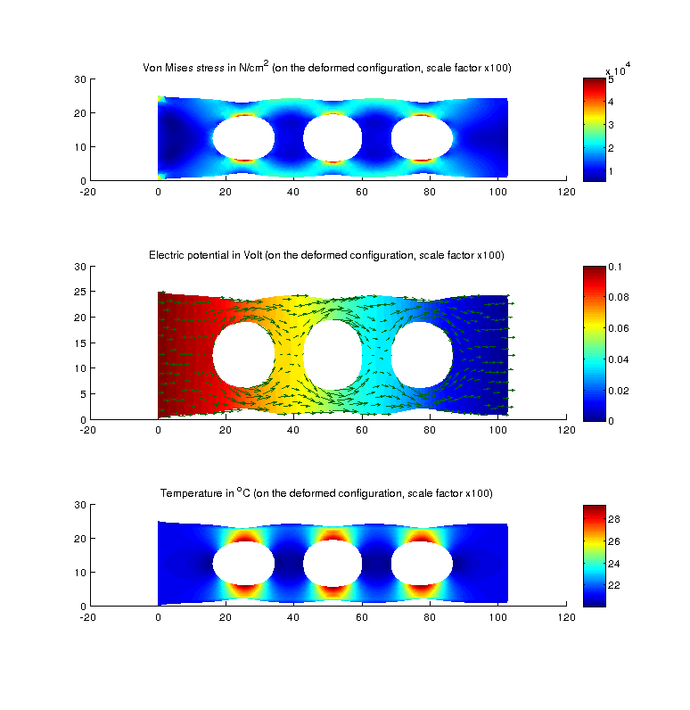
Plot of the solution.